Excel: Displaying Autofilter Criteria

Edit: 19/3/2009. Updated with instructions for adding autofilter with Excel Office 2007 and before.

I love AutoFilter in Excel: it allows you to very easily sort or hide data in various ways.

Excel Office Pre 2007: Data > Filter > AutoFilter.

Excel Office 2007: Home (on Ribbon) > click Sort & Filter > Filter. See Tables Part 4: AutoFilter improvements: much more than just multi-select for more info.

The problem is that for complicated spreadsheets, it isn't always easy to tell what filters you have applied.

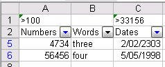
The above image indicates that the Numbers column is filtered by having that downward pointing triangle shaded blue. With a spreadsheet of 5, 10 or more columns, it is really hard to work out which of those small arrows are shaded. Worse, I can never remember exactly what filter I applied to each column.

What I do now is put a macro into the spreadsheet and a formula into the row above my headings that will show what filters have been applied i.e. display the AutoFilter criteria.

1. Open your spreadsheet and press Alt+F11 to open the Microsoft Visual Basic Editor.
2. Right click on the VBAProject entry for your spreadsheet (the spreadsheet file name is in brackets after VBAProject) > select Insert > Module.
3. In the new pane that opens to the right, make sure that (General) is selected in the drop-down at top left. Then copy and paste Stephen Bullen's macro into the VB Editor, like so (the code is below the image).

   Here is the macro code.

   Function FilterCriteria(Rng As Range) As String
       'By Stephen Bullen
       Dim Filter As String
       Filter = ""
       On Error GoTo Finish
       With Rng.Parent.AutoFilter
           If Intersect(Rng, .Range) Is Nothing Then GoTo Finish
           With .Filters(Rng.Column - .Range.Column + 1)
               If Not .On Then GoTo Finish
               Filter = .Criteria1
               Select Case .Operator
                   Case xlAnd
                       Filter = Filter & " AND " & .Criteria2
                   Case xlOr
                       Filter = Filter & " OR " & .Criteria2
               End Select
           End With
       End With
   Finish:
       FilterCriteria = Filter
   End Function
   

4. Close the VB Editor and go back to the spreadsheet.
5. Insert a new row above the headings by putting the cursor into any heading cell and selecting from the menu bar: Insert > Rows.
6. For each column that you wish to display the filter criteria for, go to the now empty row above the heading, press F2 in the cell and paste in this formula:

   =FilterCriteria(A2)&LEFT(SUBTOTAL(9,A5:A200),0)

   Correct A2 so that it correctly refers to the heading cell underneath the formula.

   You could put in just the function call by itself: =FilterCriteria(A2), but this doesn't automatically update the cell every time you change a filter. To make the formula update every time you change a filter, we add a dummy function LEFT(SUBTOTAL(9,A5:A200),0) that doesn't harm anything, just makes the spreadsheet re-evaluate the filter display whenever the filter is changed i.e. the calculation performed won't slow anything down and won't change anything displayed in the spreadsheet.

   Now, I can easily tell what AutoFilter criteria apply to my spreadsheet!

   

   Of course, there is an important disadvantage to this approach: you are putting a macro into your document, and Excel security settings apply. If the document is intended for wide distribution, consider carefully just how necessary this functionality is. Check your security settings (Tools > Macro > select Security Level tab in MS Excel 2003 and earlier). If the setting is Medium, the user will be asked whether they want to enable macros every single time they open the file. If the setting is above Medium, the macro will simply be ignored and the formula may display an error in each cell, since the function is calling a macro that isn't loaded. If the document is going to people you don't know, they may be very suspicious of a new document opening with a security warning! You can sign the macro, but that is not a trivial thing to do, at least the first time - and still requires the user to trust your signature.

7. Freeze your panes! But wait! There's more! If I have a spreadsheet complicated enough to need AutoFilter, it will probably have more than enough data to fill a single screen, which means that scrolling down makes the headings (and AutoFilter criteria display) disappear. Before you actually apply any filtering, put the cursor into the left-most cell just below the headings i.e. cell A3 in those images above. Then select on the menu bar Window > Freeze Panes. Now you can scroll down as far as you like and the first two rows will remain visible at the top.

Pages that helped me make this entry.

• Thanks to Dave Peterson on the microsoft.public.excel.misc Google group.
• Thanks to Stephen Bullen for his Excel User Tip Displaying AutoFilter criteria (a.k.a. Displaying AutoFilter Criteria on The Spreadsheet Page).
• David McRitchie's introduction to macros in this article: Getting Started with Macros and User Defined Functions.
• Debra Dalgleish's notes on how to implement macros in this Contextures article: Excel -- VBA -- Adding Code to a Workbook.
• Ron de Bruin's intro to macros, with this article: Where do I paste the code that I want to use in my workbook.
• This MSDN Blog entry on Microsoft Excel explains how to use Auto-filter in Excel Office 2007: Tables Part 4: AutoFilter improvements: much more than just multi-select.